This page was generated from: notebooks/nanopores/how_to_generate_a_tetrahedral_mesh_from_3d_nanopores_data.ipynb
[1]:
%load_ext autoreload
%autoreload 2
%config InlineBackend.rc = {'figure.figsize': (10,6)}
%matplotlib inline
Generate a 3D tetrahedral mesh
This notebook shows how to mesh a 3D volume:
Load and visualize a volume
Apply image filters and segment image
Generate a 3D surface mesh
Visualize and export the mesh to other formats
[2]:
import pyvista as pv
from skimage import filters
import numpy as np
Load and vizualize the data
This example uses nanopore sample data from nanomesh.data.
If you want to use your own data, any numpy array can be passed to into a `Image <https://nanomesh.readthedocs.io/en/latest/nanomesh.volume.html#nanomesh.volume.Volume>`__ object. Data stored as .npy can be loaded using Image.load().
[3]:
from nanomesh import Volume
from nanomesh.data import nanopores3d
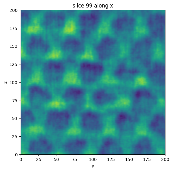
data = nanopores3d()
vol = Volume(data)
vol.show_slice()
[3]:
<nanomesh.image._utils.SliceViewer at 0x22bf619e280>
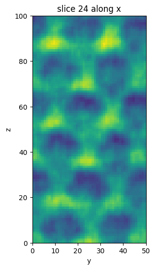
For this example, select a subvolume using .select_subvolume and downscale the image to keep the cpu times in check.
[4]:
from skimage.transform import rescale

subvol = vol.select_subvolume(
    ys=(0, 100),
    xs=(0, 100),
).apply(rescale, scale=0.5)
subvol.show_slice()
[4]:
<nanomesh.image._utils.SliceViewer at 0x22bfd514490>
Nanomesh makes use of `itkwidgets <https://github.com/InsightSoftwareConsortium/itkwidgets>`__ to render the volumes.
[5]:
subvol.show()
Filter and segment the data
Image segmentation is a way to label the pixels of different regions of interest in an image. In this example, we are interested in separating the bulk material (Si) from the nanopores. In the image, the Si is bright, and the pores are dark.
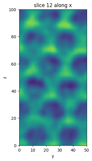
First, we apply a `gaussian filter <https://scikit-image.org/docs/dev/api/skimage.filters.html#skimage.filters.gaussian>`__ to smooth out some of the image noise to get a cleaner segmentation.
[6]:
subvol_gauss = subvol.gaussian(sigma=1)
subvol_gauss.show_slice(x=12)
[6]:
<nanomesh.image._utils.SliceViewer at 0x22b83843c40>
scikit-image contains a useful function to try all threshold finders on the data. These methods analyse the contrast histogram and try to find the optimal value to separate which parts of the image belong to each domain.
Since the function only works on a single slice, we first select a slice using the .select_plane method.
[7]:
from skimage import filters

plane = subvol_gauss.select_plane(x=12)
plane.try_all_threshold(figsize=(5, 10))
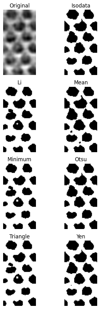
We will use the li method, because it gives nice separation.
The threshold value is used to segment the image using `np.digitize <https://numpy.org/doc/stable/reference/generated/numpy.digitize.html#numpy-digitize>`__.
[8]:
subvol_seg = subvol_gauss.binary_digitize(threshold='minimum')
subvol_seg = subvol_seg.invert_contrast()
subvol_seg.show_slice()
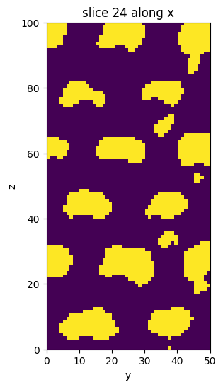
[8]:
<nanomesh.image._utils.SliceViewer at 0x22b83f31fd0>
Generate 3d tetragonal mesh
Meshes can be generated using the Mesher class. Meshing consists of two steps:
Contour finding (using the
`marching_cubes<https://scikit-image.org/docs/dev/api/skimage.measure.html#skimage.measure.marching_cubes>`__ functionTriangulation (using the
`tetgen<https://tetgen.pyvista.org/>`__ library)
Mesher requires a segmented image. generate_contour() wraps all domains of the image corresponding to that label. Here, 1 corresponds to the bulk (Si) material.
Meshing options are defined in the tetgen documentation. These can be specified using the opts parameter. The default options are opts='-pAq1.2:
-A: Assigns attributes to tetrahedra in different regions.-p: Tetrahedralizes a piecewise linear complex (PLC).-q: Refines mesh (to improve mesh quality).
Also useful:
-a: Applies a maximum tetrahedron volume constraint. Don’t make-atoo small, or the algorithm will take a very long time to complete. If this parameter is left out, the triangles will keep growing without limit.
[9]:
%%time

from nanomesh import Mesher

mesher = Mesher(subvol_seg)
mesher.generate_contour()
mesh = mesher.tetrahedralize(opts='-pAq')
Wall time: 11.4 s
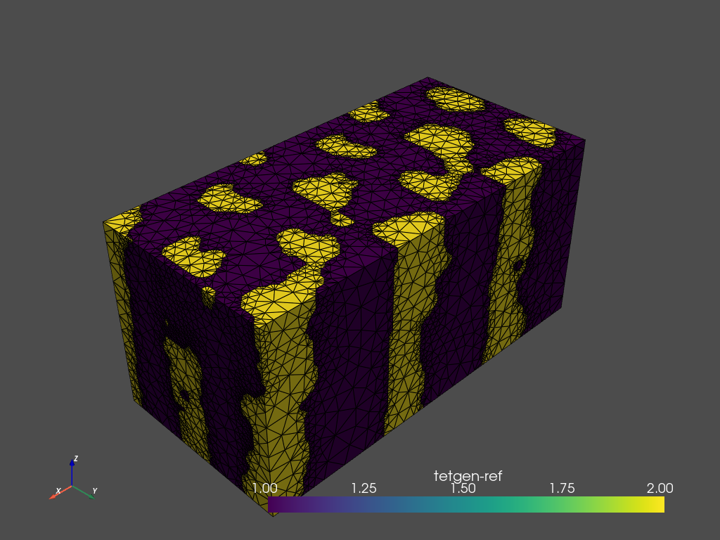
Tetrahedralization returns a TetraMesh dataclass that can be used for various operations, for example showing the result using itkwidgets:
[10]:
mesh.plot_pyvista(jupyter_backend='static', show_edges=True)
Using region markers
By default, the region attributes are assigned automatically by tetgen. Tetrahedra in each enclosed region will be assigned a new label sequentially.
Region markers are used to assign attributes to tetrahedra in different regions. After tetrahedralization, the region markers will ‘flood’ the regions up to the defined boundaries. The elements of the resulting mesh are marked according to the region they belong to (tetras.metadata['tetgenRef'].
You can view the existing region markers by looking at the .region_markers attribute on the contour.
[11]:
mesher.contour.region_markers
[11]:
RegionMarkerList(
    RegionMarker(label=1, point=(49, 17, 29), name='background', constraint=0),
    RegionMarker(label=2, point=(7, 14, 20), name='feature', constraint=0),
    RegionMarker(label=2, point=(7, 37, 20), name='feature', constraint=0),
    RegionMarker(label=2, point=(35, 36, 32), name='feature', constraint=0),
    RegionMarker(label=2, point=(26, 3, 39), name='feature', constraint=0),
    RegionMarker(label=1, point=(21.6, 48.6, 24.066666666666666), name='background', constraint=0),
    RegionMarker(label=2, point=(43, 12, 40), name='feature', constraint=0),
    RegionMarker(label=2, point=(70, 34, 35), name='feature', constraint=0),
    RegionMarker(label=1, point=(53, 23, 48), name='background', constraint=0),
    RegionMarker(label=1, point=(54, 23, 49), name='background', constraint=0),
    RegionMarker(label=2, point=(61, 2, 21), name='feature', constraint=0),
    RegionMarker(label=2, point=(78, 10, 32), name='feature', constraint=0),
    RegionMarker(label=2, point=(81, 24, 34), name='feature', constraint=0),
    RegionMarker(label=2, point=(96, 23, 22), name='feature', constraint=0),
    RegionMarker(label=2, point=(97, 3, 36), name='feature', constraint=0),
    RegionMarker(label=2, point=(90.42857142857143, 23.571428571428573, 0.42857142857142855), name='feature', constraint=0),
    RegionMarker(label=1, point=(91, 46, 0), name='background', constraint=0),
    RegionMarker(label=2, point=(99, 34, 47), name='feature', constraint=0),
    RegionMarker(label=1, point=(99, 22, 16), name='background', constraint=0)
)
It is possible to set your own attributes using the region_markers parameter. These are a list of RegionMarker objects stored in a RegionMarkerList container. You can define your own, or you can use the methods on the mesher.contour.region_markers attribute.
For example, to relabel the pores sequentially:
[12]:
mesher.contour.region_markers = mesher.contour.region_markers.label_sequentially(
    2, fmt_name='pore{}')
mesher.contour.region_markers
[12]:
RegionMarkerList(
    RegionMarker(label=1, point=(49, 17, 29), name='background', constraint=0),
    RegionMarker(label=3, point=(7, 14, 20), name='pore3', constraint=0),
    RegionMarker(label=4, point=(7, 37, 20), name='pore4', constraint=0),
    RegionMarker(label=5, point=(35, 36, 32), name='pore5', constraint=0),
    RegionMarker(label=6, point=(26, 3, 39), name='pore6', constraint=0),
    RegionMarker(label=1, point=(21.6, 48.6, 24.066666666666666), name='background', constraint=0),
    RegionMarker(label=7, point=(43, 12, 40), name='pore7', constraint=0),
    RegionMarker(label=8, point=(70, 34, 35), name='pore8', constraint=0),
    RegionMarker(label=1, point=(53, 23, 48), name='background', constraint=0),
    RegionMarker(label=1, point=(54, 23, 49), name='background', constraint=0),
    RegionMarker(label=9, point=(61, 2, 21), name='pore9', constraint=0),
    RegionMarker(label=10, point=(78, 10, 32), name='pore10', constraint=0),
    RegionMarker(label=11, point=(81, 24, 34), name='pore11', constraint=0),
    RegionMarker(label=12, point=(96, 23, 22), name='pore12', constraint=0),
    RegionMarker(label=13, point=(97, 3, 36), name='pore13', constraint=0),
    RegionMarker(label=14, point=(90.42857142857143, 23.571428571428573, 0.42857142857142855), name='pore14', constraint=0),
    RegionMarker(label=1, point=(91, 46, 0), name='background', constraint=0),
    RegionMarker(label=15, point=(99, 34, 47), name='pore15', constraint=0),
    RegionMarker(label=1, point=(99, 22, 16), name='background', constraint=0)
)
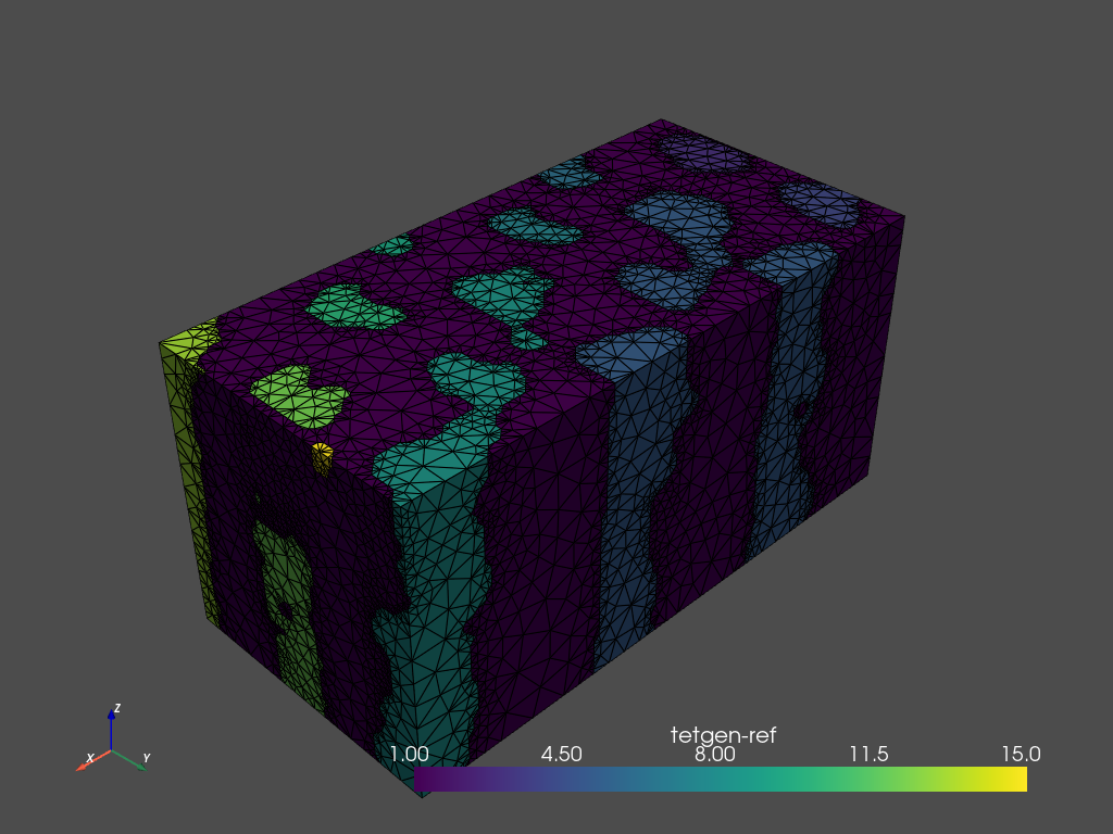
Then re-run tetrahedralization.
[13]:
%%time
import numpy as np

mesh = mesher.tetrahedralize(opts='-pAq')

for label in mesher.contour.region_markers.labels:
    num = np.sum(mesh.cell_data['tetgen:ref'] == label)
    print(f'{num} tetrahedra with attribute `{label}`')
0 tetrahedra with attribute `1`
0 tetrahedra with attribute `3`
0 tetrahedra with attribute `4`
0 tetrahedra with attribute `5`
0 tetrahedra with attribute `6`
0 tetrahedra with attribute `7`
0 tetrahedra with attribute `8`
0 tetrahedra with attribute `9`
0 tetrahedra with attribute `10`
0 tetrahedra with attribute `11`
0 tetrahedra with attribute `12`
0 tetrahedra with attribute `13`
0 tetrahedra with attribute `14`
0 tetrahedra with attribute `15`
Wall time: 10.6 s
Note that all connected regions have a different label now.
[14]:
mesh.plot_pyvista(jupyter_backend='static', show_edges=True)
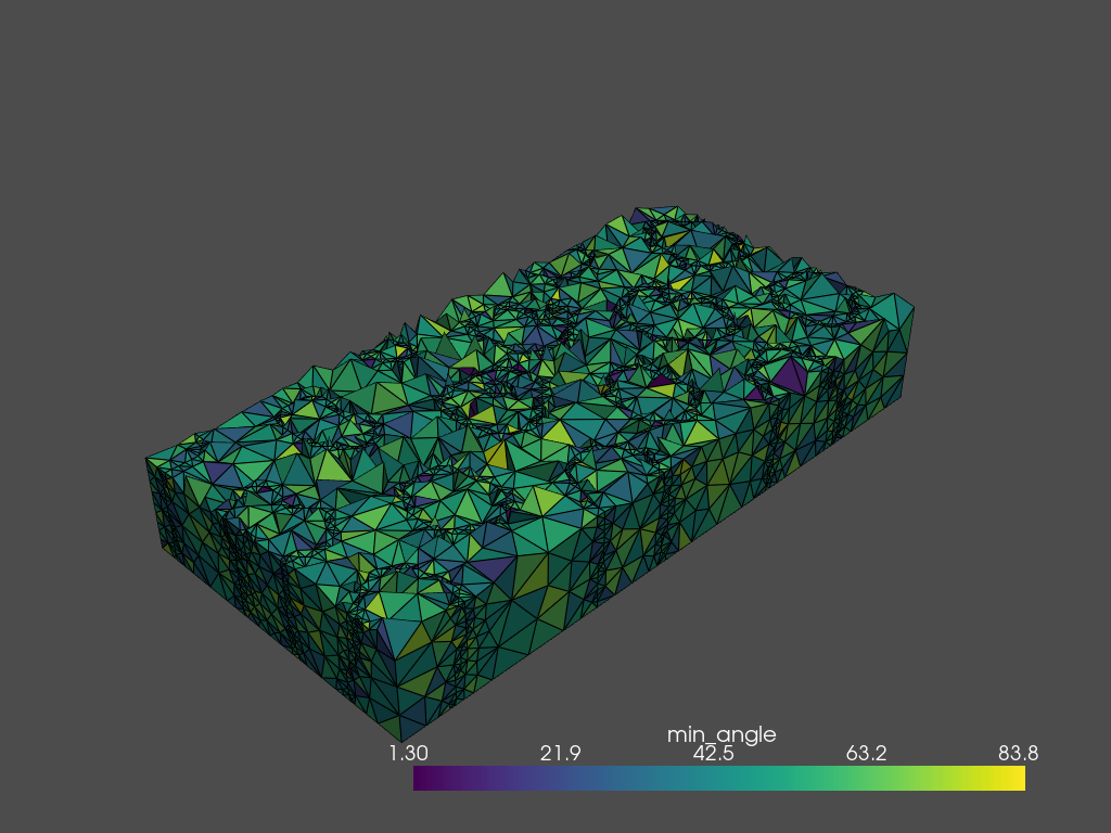
Mesh evaluation
The mesh can be evaluated using the metrics module. This example shows how to calculate all metrics and plot them on a section through the generated mesh.
[15]:
from nanomesh import metrics

tetra_mesh = mesh.get('tetra')

metrics_dict = metrics.calculate_all_metrics(tetra_mesh, inplace=True)
metrics_dict
[15]:
{'area': array([-1., -1., -1., ..., -1., -1., -1.]),
 'aspect_frobenius': array([1.46452917, 2.04351861, 1.31419018, ..., 1.24877255, 1.27624853,
        1.20117597]),
 'aspect_ratio': array([1.9706523 , 2.49095694, 1.58044016, ..., 1.61021965, 1.6569529 ,
        1.39241754]),
 'condition': array([1.41130959, 1.89977748, 1.38619841, ..., 1.21747874, 1.30710408,
        1.23581107]),
 'max_angle': array([-1., -1., -1., ..., -1., -1., -1.]),
 'min_angle': array([50.30584653, 44.91047692, 35.30258965, ..., 50.62900397,
        44.54930012, 56.87243773]),
 'radius_ratio': array([1.72076427, 2.03911704, 1.38371963, ..., 1.31649536, 1.52786183,
        1.2530299 ]),
 'scaled_jacobian': array([0.33375202, 0.15093825, 0.5137658 , ..., 0.46537578, 0.5617628 ,
        0.62871815]),
 'shape': array([0.6828133 , 0.48935204, 0.76092488, ..., 0.80078634, 0.78354645,
        0.83251749]),
 'relative_size_squared': array([0., 0., 0., ..., 0., 0., 0.]),
 'shape_and_size': array([0., 0., 0., ..., 0., 0., 0.]),
 'distortion': array([1., 1., 1., ..., 1., 1., 1.]),
 'max_min_edge_ratio': array([1.97883817, 2.94263845, 1.85817686, ..., 1.60563934, 1.71561122,
        1.26040033])}
Using the .plot_submesh() method, any array that is present in the metadata can be plotted. plot_submesh() is flexible, in that it can show a slice through the mesh as defined using index, along, and invert. Extra keyword arguments, such as show_edges and lighting are passed on to `Plotter.add_mesh() <https://docs.pyvista.org/api/plotting/_autosummary/pyvista.Plotter.add_mesh.html?highlight=add_mesh>`__.
[16]:
tetra_mesh.plot_submesh(
    along='x',
    index=15,
    scalars='min_angle',
    show_edges=True,
    lighting=True,
    backend='static',
)
[16]:
<pyvista.plotting.plotting.Plotter at 0x22b869b8d30>
Interoperability
The TetraMesh object can also be used to convert to various other library formats, such as:
`trimesh.open3d<http://www.open3d.org/docs/release/python_api/open3d.geometry.TetraMesh.html#open3d.geometry.TetraMesh>`__`pyvista.UnstructuredGrid<https://docs.pyvista.org/examples/00-load/create-unstructured-surface.html>`__`meshio.Mesh<https://docs.pyvista.org/examples/00-load/create-unstructured-surface.html>`__
To save the data, use the .write method. This is essentially a very thin wrapper around meshio, equivalent to meshio_mesh.write(...).
[17]:
tetra_mesh.write('volume_mesh.msh', file_format='gmsh22', binary=False)
Warning: Appending zeros to replace the missing physical tag data.
Warning: Appending zeros to replace the missing geometrical tag data.