This page was generated from: notebooks/nanopores/how_to_generate_a_triangle_mesh_from_a_2d_nanopore_data.ipynb
[1]:
%load_ext autoreload
%autoreload 2
%config InlineBackend.rc = {'figure.figsize': (10,6)}
%matplotlib inline
Generate a 2D triangular mesh
This notebook shows how to mesh a 2D image:
Load and visualize a volume
Select a plane from a volume
Apply image filters and segment an image
Generate a 2D triangle mesh
Visualize and export the mesh to other formats
Load and vizualize the data
This example uses nanopore sample data from nanomesh.data.
If you want to use your own data, any numpy array can be passed to into a `Volume <https://nanomesh.readthedocs.io/en/latest/nanomesh.volume.html#nanomesh.volume.Volume>`__ object. Data stored as .npy can be loaded using Volume.load().
[2]:
from nanomesh import Image
from nanomesh.data import nanopores3d

data = nanopores3d()

vol = Image(data)
vol.show_slice()
[2]:
<nanomesh.image._utils.SliceViewer at 0x1739c340fa0>
Nanomesh makes use of `itkwidgets <https://github.com/InsightSoftwareConsortium/itkwidgets>`__ to render the volumes.
[3]:
vol.show()
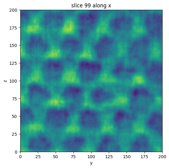
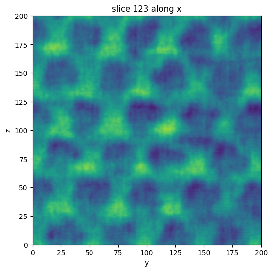
There is also a simple matplotlib based viewer to plot the slices of the volume. The sliders can be used to select different directions and slice numbers. Optionally, the index of the first slice can be specified directly using, for example, x=123.
[4]:
vol.show_slice(x=123)
[4]:
<nanomesh.image._utils.SliceViewer at 0x173a4d50c70>
Select plane from volume
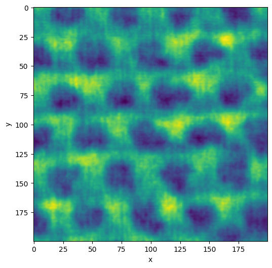
Select single plane from the volume using the .select_volume method. In this case, we select slice #161 along the x-axis. The slice is loaded into a `Plane <https://nanomesh.readthedocs.io/en/latest/nanomesh.image.html#nanomesh.image.Plane>`__ object.
[5]:
plane = vol.select_plane(x=161)
plane.show()
[5]:
<AxesSubplot:xlabel='x', ylabel='y'>
Filter and segment the data
Image segmentation is a way to label the pixels of different regions of interest in an image. In this example, we are interested in separating the bulk material (Si) from the nanopores. In the image, the Si is bright, and the pores are dark.
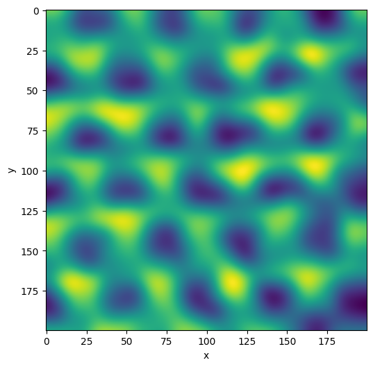
First, we apply a `gaussian filter <https://scikit-image.org/docs/dev/api/skimage.filters.html#skimage.filters.gaussian>`__ to smooth out some of the image noise to get a cleaner segmentation.
Note: The code below is essentially short-hand for plane_gauss = plane.apply(skimage.filters.gaussian, sigma=5). apply can be used for any operation that works on an array, i.e. from numpy, scipy.ndimage or scikit-image. If the output is a numpy array of the same dimensions, a Image object is returned. Anything else, and it will return the direct result of the function.
[6]:
plane_gauss = plane.gaussian(sigma=5)
plane_gauss.show()
[6]:
<AxesSubplot:xlabel='x', ylabel='y'>
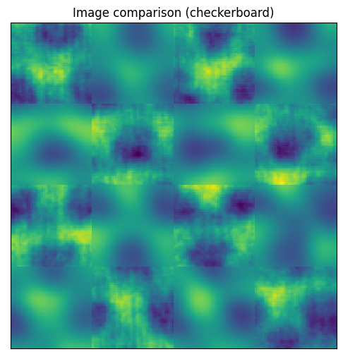
Use the compare_with_other method to check out the difference:
[7]:
plane.compare_with_other(plane_gauss)
[7]:
<AxesSubplot:title={'center':'Image comparison (checkerboard)'}>
scikit-image contains a useful function to try all threshold finders on the data. These methods analyse the contrast histogram and try to find the optimal value to separate which parts of the image belong to each domain. The method below is a shortcut to this function.
Note that it is always possible to define your own threshold.
[8]:
plane_gauss.try_all_threshold(figsize=(5, 10))
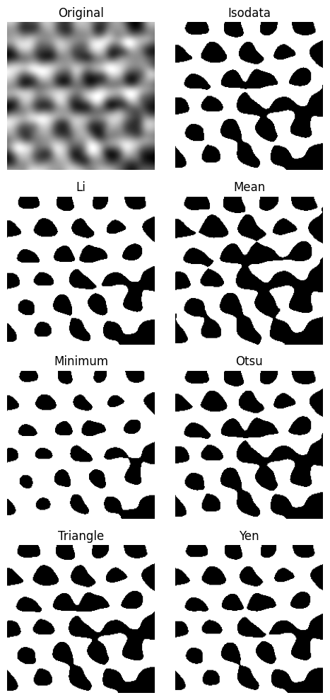
We continue with the li method, because it gives a result with nice separation.
[9]:
thresh = plane_gauss.threshold('li')
thresh
[9]:
0.45123855199826957
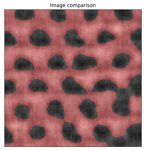
Check how the segmented image compares to the original.
[10]:
segmented = plane_gauss.digitize(bins=[thresh])
plane.compare_with_digitized(segmented)
[10]:
<AxesSubplot:title={'center':'Image comparison'}>
Generate mesh
Meshes are generated using the Mesher2D class. Meshing consists of two steps:
Contour finding (using the
`find_contours<https://scikit-image.org/docs/dev/api/skimage.measure.html#skimage.measure.find_contours>`__ functionTriangulation (using the
`triangle<https://rufat.be/triangle/>`__ library)
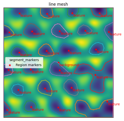
Contour finding uses the marching cubes algorithm to wrap all the pores in a polygon. max_edge_dist=5 splits up long edges in the contour, so that no two points are further than 5 pixels apart. level is directly passed to find_contours and specifies the level at which the contour is generated. In this case, we set it to the threshold value determined above.
[11]:
from nanomesh import Mesher2D

mesher = Mesher2D(plane_gauss)
mesher.generate_contour(max_edge_dist=5, level=thresh)

mesher.plot_contour()
[11]:
<AxesSubplot:title={'center':'line mesh'}>
The next step is to use the contours to initialize triangulation.
Triangulation options can be specified through the opts keyword argument. This example uses q30 to generate a quality mesh with angles > 30°, and a100 to set a maximum triangle size of 100 pixels. For more options, see here.
[12]:
mesh = mesher.triangulate(opts='q30a100')
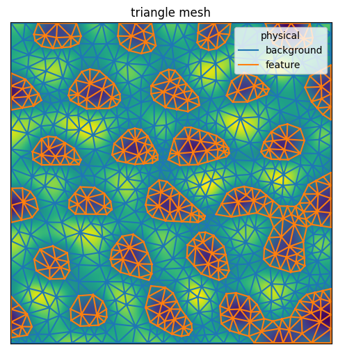
Triangulation returns a MeshContainer dataclass that can be used for various operations, for example comparing it with the original image:
[13]:
plane_gauss.compare_with_mesh(mesh)
[13]:
<AxesSubplot:title={'center':'triangle mesh'}>
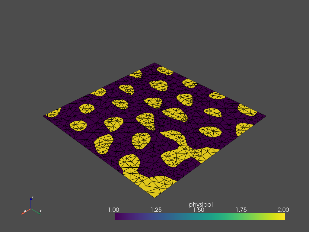
Or, showing the an interactive plot using pyvista:
(Use .plot_itk() for an interactive view)
[14]:
mesh.plot_pyvista(jupyter_backend='static', show_edges=True)
Field data
Field data can be used to associate names with the values in the cell data. These are shown in the legend of mesh data (i.e. in the plots above). The field data is stored in the .field_data attribute. Because the data are somewhat difficult to use in this state, the properties .field_to_number and .number_to_field can be used to access the mapping per cell type.
[15]:
mesh.number_to_field
[15]:
mappingproxy({'triangle': mappingproxy({2: 'feature', 1: 'background'})})
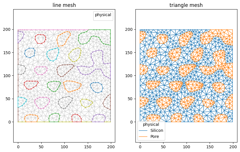
To update the values, you can update .field_data directory, or use .set_field_data. Note that field names are shared between cell types. For example, to relabel the cells data:
[16]:
mesh.set_field_data('triangle', {1: 'Silicon', 2: 'Pore'})
Plotting the mesh now shows the fields in the legend. Note that the fields are also saved when exported to a format that supports them (e.g. gmsh).
[17]:
mesh.plot(lw=1, color_map={0: 'lightgray'})
[17]:
(<AxesSubplot:title={'center':'line mesh'}>,
 <AxesSubplot:title={'center':'triangle mesh'}>)
Interoperability
The MeshContainer object can also be used to convert to various other library formats, such as:
`trimesh.Trimesh<https://trimsh.org/trimesh.base.html#trimesh.base.Trimesh>`__`pyvista.UnstructuredGrid<https://docs.pyvista.org/examples/00-load/create-unstructured-surface.html>`__`meshio.Mesh<https://docs.pyvista.org/examples/00-load/create-unstructured-surface.html>`__
First, we must extract the triangle data:
[18]:
triangle_mesh = mesh.get('triangle')

pv_mesh = triangle_mesh.to_pyvista_unstructured_grid()
trimesh_mesh = triangle_mesh.to_trimesh()
meshio_mesh = triangle_mesh.to_meshio()
To save the data, use the .write method. This is essentially a very thin wrapper around meshio, equivalent to meshio.write(...).
[19]:
mesh.write('out.msh', file_format='gmsh22', binary=False)
Warning: Appending zeros to replace the missing geometrical tag data.