This page was generated from: notebooks/examples/how_to_generate_a_triangle_mesh_from_a_2d_image.ipynb
[1]:
%load_ext autoreload
%autoreload 2
%config InlineBackend.rc = {'figure.figsize': (10,6)}
%matplotlib inline
Generate a 2D triangular mesh
This notebook shows how to mesh a 2D image:
Load and visualize a 2D data image
Generate a 2D triangle mesh
Visualize the mesh
Relabel the regions
Export the mesh to other formats
Load and vizualize the data
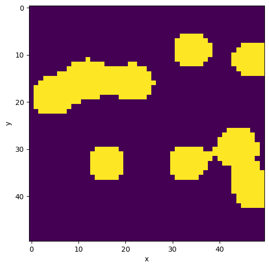
This example uses generated sample data from nanomesh.data.
If you want to use your own data, any (2D) numpy array can be passed to into a `Image <https://nanomesh.readthedocs.io/en/latest/nanomesh.plane.html#nanomesh.plane.Plane>`__ object. Data stored as .npy can be loaded using Image.load().
[2]:
from nanomesh import Image
from nanomesh.data import binary_blobs2d

data = binary_blobs2d(seed=12345)

plane = Image(data)
plane.show()
[2]:
<AxesSubplot:xlabel='x', ylabel='y'>
Generate mesh
Meshes are generated using the Mesher2D class. Meshing consists of two steps:
Contour finding (using the
`find_contours<https://scikit-image.org/docs/dev/api/skimage.measure.html#skimage.measure.find_contours>`__ functionTriangulation (using the
`triangle<https://rufat.be/triangle/>`__ library)
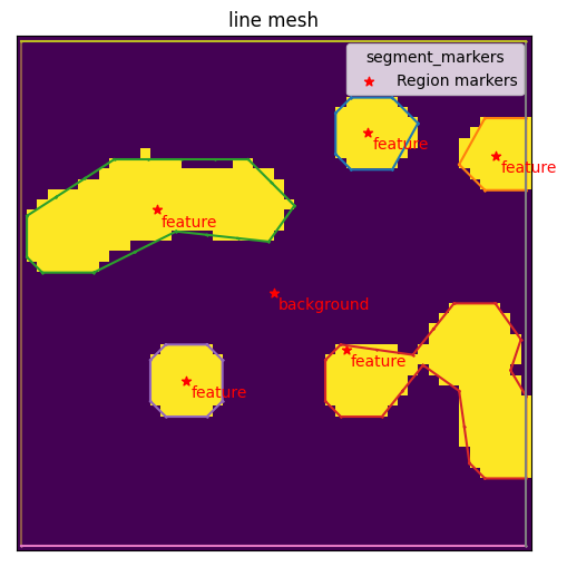
Contour finding uses the marching cubes algorithm to wrap all the pores in a polygon. max_edge_dist=5 splits up long edges in the contour, so that no two points are further than 5 pixels apart. level is directly passed to find_contours and specifies the level at which the contour is generated. In this case, we set it to the threshold value determined above.
[3]:
from nanomesh import Mesher2D

mesher = Mesher2D(plane)
mesher.generate_contour(max_edge_dist=3)

mesher.plot_contour()
[3]:
<AxesSubplot:title={'center':'line mesh'}>
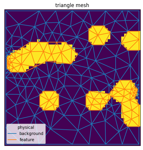
The next step is to use the contours to initialize triangulation.
Triangulation options can be specified through the opts keyword argument. This example uses q30 to generate a quality mesh with angles > 30°, and a100 to set a maximum triangle size of 100 pixels. For more options, see here.
[4]:
mesh = mesher.triangulate(opts='q30a100')
Triangulation returns a MeshContainer dataclass that can be used for various operations, for example comparing it with the original image:
[5]:
plane.compare_with_mesh(mesh)
[5]:
<AxesSubplot:title={'center':'triangle mesh'}>
Region markers
By default, regions are split up in the background and features. Feature regions are grouped by the label 1.
[6]:
mesher.contour.region_markers
[6]:
RegionMarkerList(
    RegionMarker(label=2, point=(8.857142857142858, 33.642857142857146), name='feature', constraint=0),
    RegionMarker(label=2, point=(11.2, 46.1), name='feature', constraint=0),
    RegionMarker(label=2, point=(16.40277777777778, 13.152777777777779), name='feature', constraint=0),
    RegionMarker(label=2, point=(30.02357502501259, 31.509054204728493), name='feature', constraint=0),
    RegionMarker(label=2, point=(33.0, 16.0), name='feature', constraint=0),
    RegionMarker(label=1, point=(24.5, 24.5), name='background', constraint=0)
)
To label regions sequentially, set group_regions=False:
[7]:
mesher = Mesher2D(plane)
mesher.generate_contour(max_edge_dist=3, group_regions=False)

mesher.plot_contour()
[7]:
<AxesSubplot:title={'center':'line mesh'}>
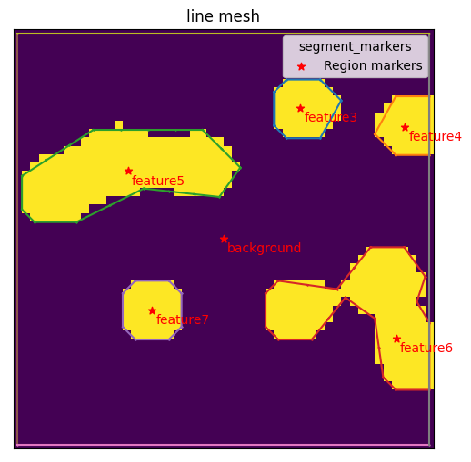
Notice that each feature has been given a unique name:
[8]:
mesher.contour.region_markers
[8]:
RegionMarkerList(
    RegionMarker(label=3, point=(8.857142857142858, 33.642857142857146), name='feature3', constraint=0),
    RegionMarker(label=4, point=(11.2, 46.1), name='feature4', constraint=0),
    RegionMarker(label=5, point=(16.40277777777778, 13.152777777777779), name='feature5', constraint=0),
    RegionMarker(label=6, point=(36.40467875597856, 45.03515883059761), name='feature6', constraint=0),
    RegionMarker(label=7, point=(33.0, 16.0), name='feature7', constraint=0),
    RegionMarker(label=1, point=(24.5, 24.5), name='background', constraint=0)
)
These labels will assigned to each triangle in the corresponding region after triangulation. These are stored in mesh.cell_data of the MeshContainer. This container stores a single set of points, and both the line segments (LineMesh) and triangles (TriangleMesh). To extract the triangle cells only, use MeshContainer.get('triangle'). this returns a class that is simpler to work with.
The cell below shows how to use this to access the cell data for the triangle cells in the mesh.
[9]:
mesh = mesher.triangulate(opts='q30a100')
mesh.get('triangle').cell_data
[9]:
{'physical': array([1., 1., 5., 1., 1., 5., 1., 5., 5., 1., 5., 1., 5., 1., 5., 1., 1.,
        5., 5., 1., 1., 1., 5., 5., 1., 5., 1., 5., 1., 3., 3., 1., 1., 3.,
        1., 1., 4., 1., 1., 1., 3., 1., 1., 1., 1., 5., 5., 1., 1., 1., 4.,
        1., 1., 4., 1., 3., 1., 1., 5., 1., 1., 1., 7., 1., 1., 1., 1., 6.,
        7., 1., 7., 1., 7., 1., 1., 1., 1., 7., 1., 1., 6., 1., 1., 6., 1.,
        7., 1., 6., 6., 1., 6., 6., 6., 6., 1., 6., 1., 6., 6., 1., 1., 1.,
        1., 1., 6., 1., 1., 6., 6., 6., 1., 1., 1., 1., 1., 6., 6., 1., 1.,
        1., 1., 1., 1., 1., 1., 5., 1., 1., 1., 5., 1., 1., 5., 1., 5., 1.,
        1., 1., 1., 1., 5., 1., 5., 5., 5., 1., 5., 5., 5., 5., 5., 6., 1.,
        1., 1., 5., 6., 1., 6., 1., 5., 5., 1., 1., 6., 1., 1., 6., 6., 6.,
        6., 6., 6., 1., 5., 5., 6., 6., 6., 6., 6., 6., 6., 1., 6., 1., 6.,
        1., 6., 1., 1., 6., 6., 1., 1., 1., 5., 1., 1., 6., 6., 5., 5., 3.,
        3., 1., 1., 1., 1., 1., 1., 1., 1., 7., 7., 1., 1., 6., 6., 1., 1.,
        1., 6., 1., 1., 6., 6., 1., 1., 5., 5., 5., 1., 5., 1., 1., 7., 7.,
        1., 1., 6., 6., 6., 6., 1., 1., 1., 1., 1., 1., 1., 1., 1., 1., 1.,
        1., 6., 6., 1., 1., 5., 5., 1., 1., 1., 1., 1., 1., 5., 1., 5., 1.,
        1., 5., 5., 1., 1., 1., 1., 1., 1., 1., 1., 6., 6., 1., 1., 1., 1.,
        5., 5., 1., 1., 1., 1., 1., 1., 1., 1., 1., 1., 1., 1., 1., 1., 1.,
        4., 1., 1., 1., 1., 1., 1., 1., 1., 1., 1., 1., 1., 1., 1., 1., 1.,
        1., 1., 1., 1., 1., 1., 1., 1., 1., 1., 1., 1., 1., 1., 1., 1., 1.,
        1., 1., 1., 1., 1., 1., 1., 1., 1., 1., 1., 1., 1., 1., 1., 1.])}
Field data
Field data can be used to associate names with the values in the cell data. These are shown in the legend of mesh data (i.e. in the plots above). The field data is stored in the .field_data attribute. Because the data are somewhat difficult to use in this state, the properties .field_to_number and .number_to_field can be used to access the mapping per cell type.
[10]:
mesh.number_to_field
[10]:
mappingproxy({'triangle': mappingproxy({3: 'feature3',
                            4: 'feature4',
                            5: 'feature5',
                            6: 'feature6',
                            7: 'feature7',
                            1: 'background'})})
To update the values, you can update .field_data directory, or use .set_field_data. Note that field names are shared between cell types. For example, to relabel the cells data:
[11]:
fields = {}
for k, v in mesh.number_to_field['triangle'].items():
    v = v.replace('background', 'Silicon')
    v = v.replace('feature', 'Pore')
    fields[k] = v

mesh.set_field_data('triangle', fields)
mesh.number_to_field
[11]:
mappingproxy({'triangle': mappingproxy({3: 'Pore3',
                            4: 'Pore4',
                            5: 'Pore5',
                            6: 'Pore6',
                            7: 'Pore7',
                            1: 'Silicon'})})
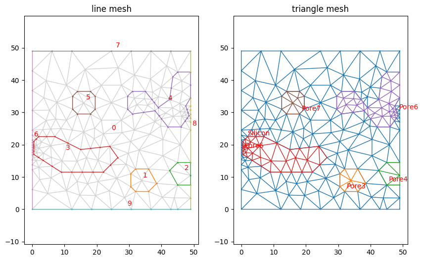
Plotting the mesh now shows the fields in the legend. Note that the fields are also saved when exported to a format that supports them (e.g. gmsh).
[12]:
mesh.plot(lw=1, color_map={0: 'lightgray'}, legend='floating')
[12]:
(<AxesSubplot:title={'center':'line mesh'}>,
 <AxesSubplot:title={'center':'triangle mesh'}>)
Interoperability
The MeshContainer object can also be used to convert to various other library formats, such as:
`trimesh.Trimesh<https://trimsh.org/trimesh.base.html#trimesh.base.Trimesh>`__`pyvista.UnstructuredGrid<https://docs.pyvista.org/examples/00-load/create-unstructured-surface.html>`__`meshio.Mesh<https://docs.pyvista.org/examples/00-load/create-unstructured-surface.html>`__
First, we must extract the triangle data:
[13]:
triangle_mesh = mesh.get('triangle')

pv_mesh = triangle_mesh.to_pyvista_unstructured_grid()
trimesh_mesh = triangle_mesh.to_trimesh()
meshio_mesh = triangle_mesh.to_meshio()
To save the data, use the .write method. This is essentially a very thin wrapper around meshio, equivalent to meshio.write(...).
[14]:
mesh.write('out.msh', file_format='gmsh22', binary=False)
Warning: Appending zeros to replace the missing geometrical tag data.