This page was generated from: notebooks/finite_elements/how_to_poisson_with_getfem.ipynb
[1]:
%config InlineBackend.rc = {'figure.figsize': (10,6)}
%matplotlib inline
Poisson equation with getfem
This example solves the Poisson problem using getfem using data generated by Nanomesh. We solve the Poisson problem \(-\Delta u = 1\) with the boundary condition \(u=0\).
This an adaptation of Python getfem demo.
Setup getfem
First, we must setup the path to the python module (link), so that getfem can be used in our Nanomesh environment.
We import getfem and generate a mesh to test if it works.
[2]:
import sys
sys.path.append('../../../getfem/interface/src/python/')

import getfem
m = getfem.Mesh('cartesian', range(0, 3), range(0,3))
print(m)
BEGIN POINTS LIST

  POINT COUNT 9
  POINT  0  0  0
  POINT  1  1  0
  POINT  2  2  0
  POINT  3  0  1
  POINT  4  1  1
  POINT  5  2  1
  POINT  6  0  2
  POINT  7  1  2
  POINT  8  2  2

END POINTS LIST


BEGIN MESH STRUCTURE DESCRIPTION

  CONVEX COUNT 4
  CONVEX 0    'GT_LINEAR_PRODUCT(GT_PK(1,1),GT_PK(1,1))'      0  1  3  4
  CONVEX 1    'GT_LINEAR_PRODUCT(GT_PK(1,1),GT_PK(1,1))'      1  2  4  5
  CONVEX 2    'GT_LINEAR_PRODUCT(GT_PK(1,1),GT_PK(1,1))'      3  4  6  7
  CONVEX 3    'GT_LINEAR_PRODUCT(GT_PK(1,1),GT_PK(1,1))'      4  5  7  8

END MESH STRUCTURE DESCRIPTION
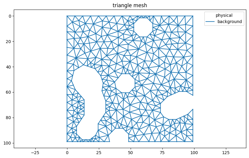
Generate some data
We use the 2D binary blobs data to generate a triangle mesh. The triangles that belong to the blobs are removed.
[3]:
from skimage.morphology import disk
from nanomesh.data import binary_blobs2d

data = binary_blobs2d(length=100, seed=96)

from nanomesh import Mesher

mesher = Mesher(data)
mesher.generate_contour(max_edge_dist=3, precision=1)
mesh = mesher.triangulate(opts='q30a25')

triangles = mesh.get('triangle')
triangles.remove_cells(label=2, key='physical')

triangles.plot()
[3]:
<AxesSubplot:title={'center':'triangle mesh'}>
Convert to getfem mesh type
We use the 2D triangulation mesh type described by passing the argument pt2D. Note that the points and cells arrays must be transposed.
[4]:
import getfem as gf

p = triangles.points.T
t = triangles.cells.T

mesh = gf.Mesh('pt2D', p, t)
mesh
[4]:
message from gf_mesh_get follow:
gfMesh object in dimension 2 with 389 points and 615 elements
Poisson’s equation
The next cell shows how to solve the Poisson equation. This code was re-used from here.
[5]:
import getfem as gf
import numpy as np

OUTER_BOUND = 1

outer_faces = mesh.outer_faces()
mesh.set_region(OUTER_BOUND, outer_faces)

sl = gf.Slice(("none",), mesh, 1)

elements_degree = 2

mfu = gf.MeshFem(mesh, 1)
mfu.set_classical_fem(elements_degree)

mim = gf.MeshIm(mesh, pow(elements_degree, 2))

F = 1.0

md = gf.Model("real")

md.add_fem_variable("u", mfu)
md.add_Laplacian_brick(mim, "u")
md.add_fem_data("F", mfu)
md.set_variable("F", np.repeat(F, mfu.nbdof()))
md.add_source_term_brick(mim, "u", "F")
md.add_Dirichlet_condition_with_multipliers(mim, "u", elements_degree - 1, OUTER_BOUND)

md.solve()
Trace 2 in getfem_models.cc, line 4401: Mass term assembly for Dirichlet condition
Trace 2 in getfem_models.cc, line 3478: Laplacian: generic matrix assembly
Trace 2 in getfem_models.cc, line 3310: Generic source term assembly
Trace 2 in getfem_models.cc, line 3321: Source term: generic source term assembly
Trace 2 in getfem_models.cc, line 4401: Mass term assembly for Dirichlet condition
[5]:
(0, 1)
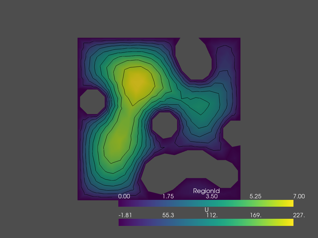
Display result using PyVista
The data can be visualized by saving to a vtk file, and loading that with PyVista.
[6]:
import pyvista as pv

U = md.variable("u")
sl.export_to_vtk("u.vtk", "ascii", mfu, U, "U")

m = pv.read("u.vtk")
contours = m.contour()

p = pv.Plotter()
p.add_mesh(m, show_edges=False)
p.add_mesh(contours, color="black", line_width=1)
p.add_mesh(m.contour(8).extract_largest(), opacity=0.1)
p.show(cpos="xy", jupyter_backend='static')