This page was generated from: notebooks/finite_elements/how_to_use_with_sfepy_horse.ipynb
[1]:
%load_ext autoreload
%autoreload 2
%config InlineBackend.rc = {'figure.figsize': (10,6)}
%matplotlib inline
Fluid dynamics with SfePy
In this notebook we recreate one of the SfePy examples using a mesh generated with Nanomesh.
The original example, describes a Laplace equation that models the flow of “dry water” around an obstacle shaped like a Citroen CX. Fluid dynamics are commonly used to model air flow around an object. We don’t have an image of a car, but let’s see how far we get with modeling aero-dynamics of a horse. :-)
Prerequisites: - Sfepy - Mayavi (optional, for one of the plots)
Load data
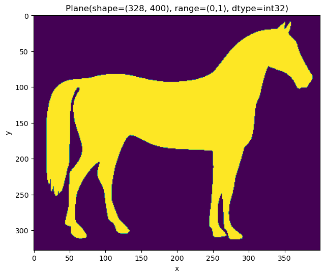
This example uses the skimage horse sample data.
The data are inverted and small gaps in the tail are filled.
[2]:
from skimage.data import horse
from nanomesh import Image
from scipy import ndimage as ndi

data = horse()

plane = Image(~data)
plane = plane.apply(ndi.binary_fill_holes).astype(int)

plane.show(title=plane)
[2]:
<AxesSubplot:title={'center':'Plane(shape=(328, 400), range=(0,1), dtype=int32)'}, xlabel='x', ylabel='y'>
Generating the mesh
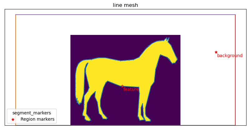
The shape of the object is simplified to reduce the number of triangles. Note that the bbox was expanded to leave some head/tail room for the partial derivatives.
[3]:
from nanomesh import Mesher
mesher = Mesher(plane)
mesher.bbox = [[ -75, -200],
[327, -200],
[327, 599],
[ -75, 599]]
mesher.generate_contour(precision=2, max_edge_dist=15)
mesher.plot_contour()
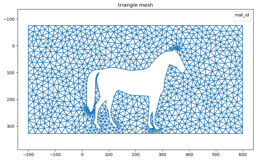
nanomesh_mesh = mesher.triangulate(opts='pAq30a300')
nanomesh_mesh.plot()
[3]:
(<AxesSubplot:title={'center':'line mesh'}>,
 <AxesSubplot:title={'center':'triangle mesh'}>)
Prepare mesh for SfePy
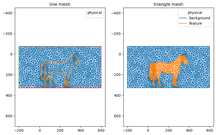
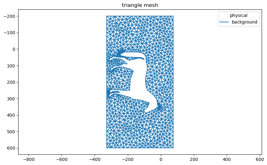
In the next cell we extract the triangle mesh and prepare the mesh for SfePy.
Remove triangles representing the horse using the
Mesh.remove_cells()method.Flip and rotate the coordinates. This ensures the mesh has the correct orientation.
[4]:
import numpy as np

triangles = nanomesh_mesh.get('triangle')
triangles.remove_cells(label=2, key='physical')

triangles.points = np.flip(triangles.points, axis=1)
triangles.points[:,1] = -triangles.points[:,1]

triangles.plot()
[4]:
<AxesSubplot:title={'center':'triangle mesh'}>
Running SfePy the easy way
At this stage, the data can also be saved to SfePy-supported data type, and run using the command-line options.
[5]:
triangles.write('horse.vtk')
VTK requires 3D points, but 2D points given. Appending 0 third component.
Running Sfepy the interactive way
To run SfePy in the Jupyter notebook, we need to set up the config interactively.
The next cell sets up the config for SfePy.
The problem_desc class essentially defines what is known as the **problem description file**.
The mesh from Nanomesh is converted using the mesh_hook.
[6]:
from sfepy.discrete.fem.meshio import UserMeshIO
from sfepy.discrete.fem import Mesh

def mesh_hook(mesh, mode):
    if mode == 'read':
        points = triangles.points

        cells = triangles.cells
        cell_data = triangles.cell_data['physical']
        cell_description = ['2_3']

        mesh = Mesh.from_data(
            'triangle',
            points,
            None,
            [cells],
            [cell_data],
            cell_description
        )
        return mesh

xmin, ymin = triangles.points.min(axis=0)
xmax, ymax = triangles.points.max(axis=0)

class problem_desc:
    __file__ = 'nanomesh'  # dummy value
    filename_mesh = UserMeshIO(mesh_hook)

    # 2D vector defining far field velocity
    v0 = np.array([
        [-1.0],
        [0.0],
    ])

    materials = {
        'm': (
            {
                'v0': v0
            },
        ),
    }

    regions = {
        'Omega': 'all',
        'Gamma_Left': (f'vertices in (x < {xmin+0.1})', 'facet'),
        'Gamma_Right': (f'vertices in (x > {xmax-0.1})', 'facet'),
        'Gamma_Top': (f'vertices in (y > {ymax-0.1})', 'facet'),
        'Gamma_Bottom': (f'vertices in (y < {ymax+0.1})', 'facet'),
        'Vertex': ('vertex in r.Gamma_Left', 'vertex'),
    }

    fields = {
        'u': ('real', 1, 'Omega', 1),
    }

    variables = {
        'phi': ('unknown field', 'u', 0),
        'psi': ('test field', 'u', 'phi'),
    }

    # these EBCS prevent the matrix from being singular, see description
    ebcs = {
        'fix': ('Vertex', {'phi.0': 0.0}),
    }

    integrals = {
        'i': 2,
    }

    equations = {
        'Laplace equation':
            """dw_laplace.i.Omega( psi, phi )
             = dw_surface_ndot.i.Gamma_Left( m.v0, psi )
             + dw_surface_ndot.i.Gamma_Right( m.v0, psi )
             + dw_surface_ndot.i.Gamma_Top( m.v0, psi )
             + dw_surface_ndot.i.Gamma_Bottom( m.v0, psi )"""
    }

    solvers = {
        'ls': ('ls.scipy_direct', {}),
        'newton': ('nls.newton', {
            'i_max': 5,
            'eps_a': 1e-16,
        }),
    }

from sfepy.base.conf import ProblemConf

conf = ProblemConf.from_module(problem_desc)
sfepy: left over: ['__module__', '__file__', 'filename_mesh', 'v0', 'materials', 'regions', 'fields', 'variables', 'ebcs', 'integrals', 'equations', 'solvers', '__dict__', '__weakref__', '__doc__', 'verbose', '_filename']
Bonus: Accessings SfePy mesh type
Now that the config has been defined, the next cell contains a little snippet to load the SfePy mesh from the config.
[7]:
from sfepy.discrete.fem import Mesh
trunk = conf.filename_mesh.get_filename_trunk()
mesh = conf.filename_mesh.read(Mesh(trunk))
mesh._set_shape_info()
mesh
[7]:
Mesh:triangle
Solving the PDE with FEM
Solving the partial differential equations with SfePy is straightforward:
[8]:
from sfepy.applications import solve_pde

problem, variables = solve_pde(conf)
sfepy: reading mesh (triangle)...
sfepy: ...done in 0.00 s
sfepy: creating regions...
sfepy:     Omega
sfepy:     Gamma_Left
sfepy:     Gamma_Right
sfepy:     Gamma_Top
sfepy:     Gamma_Bottom
sfepy:     Vertex
sfepy: ...done in 0.01 s
sfepy: equation "Laplace equation":
sfepy: dw_laplace.i.Omega( psi, phi )
             = dw_surface_ndot.i.Gamma_Left( m.v0, psi )
             + dw_surface_ndot.i.Gamma_Right( m.v0, psi )
             + dw_surface_ndot.i.Gamma_Top( m.v0, psi )
             + dw_surface_ndot.i.Gamma_Bottom( m.v0, psi )
sfepy: using solvers:
                ts: no ts
               nls: newton
                ls: ls
sfepy: updating variables...
sfepy: ...done
sfepy: setting up dof connectivities...
sfepy: ...done in 0.03 s
sfepy: matrix shape: (1038, 1038)
sfepy: assembling matrix graph...
sfepy: ...done in 0.00 s
sfepy: matrix structural nonzeros: 6644 (6.17e-01% fill)
sfepy: updating variables...
sfepy: ...done
sfepy: updating materials...
sfepy:     m
sfepy: ...done in 0.03 s
sfepy: nls: iter: 0, residual: 3.065684e+02 (rel: 1.000000e+00)
sfepy:   residual:    0.05 [s]
sfepy:     matrix:    0.00 [s]
sfepy:      solve:    0.06 [s]
sfepy: warning: linear system solution precision is lower
sfepy: then the value set in solver options! (err = 2.467691e-11 < 1.000000e-16)
sfepy: nls: iter: 1, residual: 2.633983e-11 (rel: 8.591827e-14)
sfepy:   residual:    0.00 [s]
sfepy:     matrix:    0.00 [s]
sfepy:      solve:    0.00 [s]
sfepy: nls: iter: 2, residual: 1.069554e-11 (rel: 3.488795e-14)
sfepy:   residual:    0.00 [s]
sfepy:     matrix:    0.00 [s]
sfepy:      solve:    0.00 [s]
sfepy: nls: iter: 3, residual: 9.991876e-12 (rel: 3.259265e-14)
sfepy:   residual:    0.00 [s]
sfepy:     matrix:    0.00 [s]
sfepy:      solve:    0.00 [s]
sfepy: nls: iter: 4, residual: 9.428764e-12 (rel: 3.075583e-14)
sfepy:   residual:    0.00 [s]
sfepy:     matrix:    0.00 [s]
sfepy:      solve:    0.00 [s]
sfepy: linesearch: iter 5, (9.73613e-12 < 9.42867e-12) (new ls: 1.000000e-01)
sfepy: nls: iter: 5, residual: 9.150060e-12 (rel: 2.984672e-14)
sfepy: solved in 1 steps in 0.18 seconds
Plot with Mayavi
The data can be stored to a file, and then displayed in Mayavi.
Note that this will open a new window.
[9]:
from sfepy.postprocess.viewer import Viewer

out = 'phi.vtk'

problem.save_state(out, variables)

view = Viewer(out)
view(rel_scaling=2, is_scalar_bar=True,
     is_wireframe=True, colormap='viridis')
sfepy: reading mesh (phi.vtk)...
sfepy:   number of vertices: 1039
sfepy:   number of cells:
sfepy:     2_3: 1766
sfepy: ...done in 0.01 s
sfepy: point scalars phi at [-399.5 -201.     0. ]
sfepy: range: -2.28e+03 4.74e+01 l2 norm range: 0.00e+00 2.28e+03
[9]:
<sfepy.postprocess.viewer.ViewerGUI at 0x2b438f1c450>
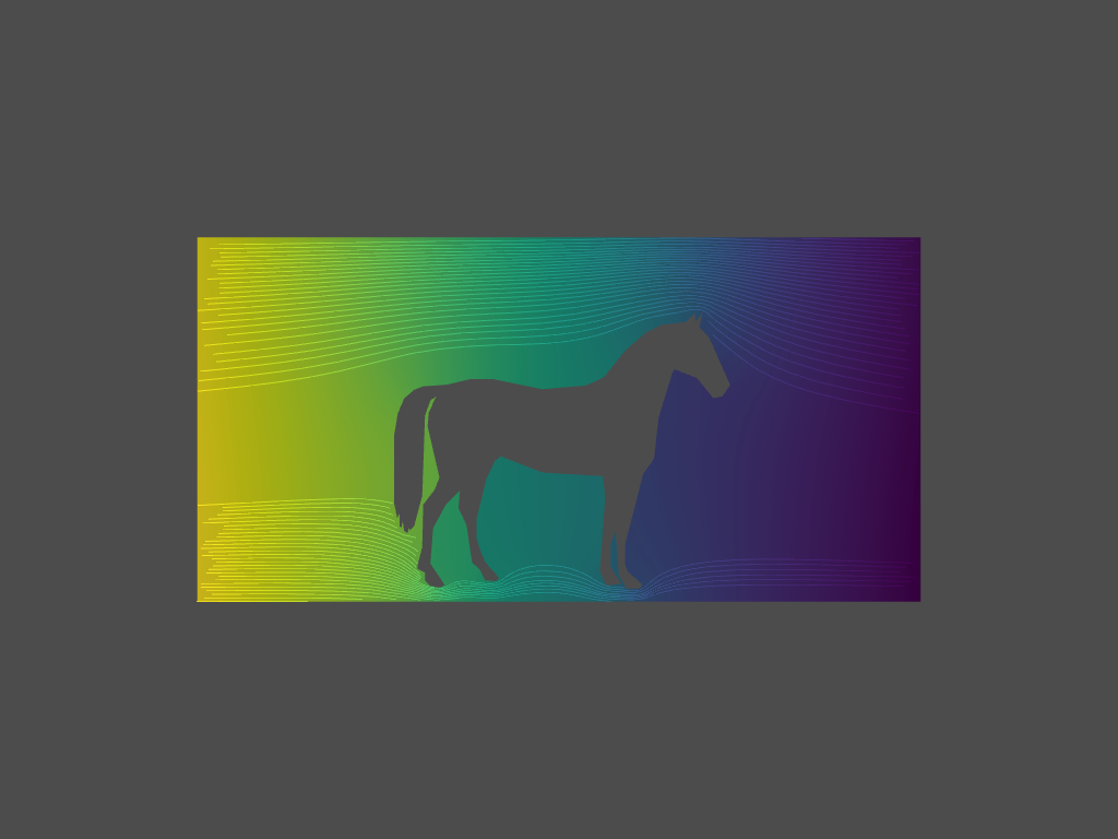
Flow plot using pyvista
To view the streamlines, we use the pv_plot function from Sfepy. This uses pyvista as the renderer.
This is normally a command-line tool, so we must mimick the plotting options.
[10]:
from resview import pv_plot

class options:
    step = 0
    view_2d = True
    position_vector = None
    fields_map = []
    fields = [
        ('phi', 'p0'),
        ('phi', 't100:p0'),
             ]
    opacity = 1.
    show_edges = False
    warp = None
    factor = 1.0
    outline = False
    color_map = None
    show_scalar_bars = False
    show_labels = False


plotter = pv_plot([out], options=options, use_cache=False)
plotter.view_xy()
plotter.show(jupyter_backend='static')
mesh from phi.vtk:
  points:  1039
  cells:   1766
  bounds:  [(-200.0, 599.0), (-327.0, 75.0), (0.0, 0.0)]
  scalars: phi, node_groups, mat_id
  steps:   1
plot 0: phi(step 0); phi(step 0)
Loading the data back into Nanomesh
The data can be loaded back into Nanomesh. Note that we must flip back the coordinates to get the correct orientation.
[11]:
from nanomesh import MeshContainer

mesh_container = MeshContainer.read(out)

mesh_container.points[:,1] = -mesh_container.points[:,1]
mesh_container.points = np.flip(mesh_container.points, axis=1)

mesh_container.plot('triangle')
[11]:
<AxesSubplot:title={'center':'triangle mesh'}>